Towards Automatic Generation of Problem Solving Techniques using a Genetic Programming Approach:
Mapping cyclic and acyclic graphs in open architecture systems
Ricardo A. Garcia Machine Listening Group, MIT Media Lab.
Date: May 11, 2000
Introduction
It would be very interesting if the user could present a "problem" to the computer, and the computer returned not just the "solution" to that problem, but also the "technique" or process that was used to arrive to the solution. Well, this is what we are trying to do now: to find a way to present problems to the computer and ask it to find a way to solve it, and specially, to give us the "method" used to solve the problem.
The method that we will discuss is called genetic programming (GP) as proposed by Koza, et al. [ 1 ] and it is meant to generate a computer program that will solve a problem given a high level statement about it, without any (or limited knowledge) of how to solve it. To make things easier, we will introduce a simple problem of training a creature in a simple world to achieve a simple goal, and discuss all the aspects that have to be taken in account in using a GP approach for this goal. Specially, it will be focused in the necessity of a good "mapping" between cyclic and acyclic graphs, a crucial point to use GP in open architecture systems.
The "toy" problem
Our goal is to design a system that shows adaptive behavior, as the behavior found in simple life form organisms.

Imagine a "creature"(triangle) in a two dimensional grid (Figure 1), with some "food" (dots) and some "poison" (asterisks). The creature needs to eat as much food as it can, and don’t eat poison at all. The creature will have some sensors (to see/smell/touch the food/poison/walls) and some actuators (to move/eat). Our goal is to find an algorithm or program that will keep alive these creatures in different environments (different "worlds" with various sizes and food/poison distributions).
We have control over the world sizes and food/poison distributions in both, the training and the testing, but we are supposed to have no control over the actual creature once the simulation is running. Also, the idea is to find an algorithm that will perform very well in different situations without changing any parameters on it (that is the adaptive part).
Solving Problems
To solve a problem in general, we must to have clear some things:
- The problem itself: well, this sound dumb, but is very important. We have to know what is the real problem that we are trying to solve. It is important to "separate" what is the knowledge that we have before solving the problem, and the knowledge that we expect to have after solving the problem. Also, all the surrounding knowledge that is related to the problem is very important. In GP this knowledge is actually the one that will help us find a solution (or at least narrow the search). By surrounding knowledge we mean the knowledge that accompanies the problem (or the solution). In the "toy" example, our knowledge is that the "evolved" creature must eat all the possible dots and not eat poison at all.
- Problem/solution architecture: the problem and the actual solution have an architecture that should be known in some instances. Usually, the problem architecture is given by the actual problem (that means that we can’t change it) but the architecture of the solution is not known (usually). If the user decides to select a particular architecture for the solution, then the task is to search for the optimal parameters to make this solution be the one that solves our particular problem. In our case, our goal is even higher, and the selection of an architecture will be part of the solution to the problem (it can be argued that it is not just a part of the solution, but the "solution" itself). By architecture, we mean the special arrangement of processing blocks, inputs, outputs, etc or what is usually called the "information flow diagram". In GP, the goal is to leave the architecture of the solution open, and make this topology be part of the solution that will be found as well as the parameters associated with the architecture. Therefore, the space to be searched is bigger (with all the allowable topologies plus all the possible parameters in each topology)
- Some way to test the solution: Every solution has to be tested under supervised conditions to "rank" it and decide if it is suitable for the problem at hand.
- Definition of Inputs and Outputs: Because if the architecture of the solution is open, we need some standard way to put information into the system and also for retrieving information. This can be seen as a "black box" system, where we don’t care about the system inside, but we have some standard interfaces to talk the box.
Open Architecture systems
The architecture of the solution of a problem, is usually selected taken in account some aspects as:
- in what kind of platform will the solution be run (i.e. in a digital computer, analog computer, an algorithm with paper and pencil, etc)
- Amount of resources available at the platform.
- Preferences in the use of resources (i.e. cost issues).
This kind of selections have to be done before attempting to give your problem to an automated problem solver, because they are too specific to your resources and intentions.
Knowing the kind of platform and the available resources narrows down the search for a solution. This solution of the problem can be presented as a special "arrangement" of functional blocks. These functional blocks are the "basic" functions or elements that are available in the selected platform. In theory, if the platform is flexible enough, there is a big possibility to arrange these blocks in some fashion that will solve our problem.
Then, the solution can be thought as the specific arrangement of the blocks (types of blocks, and connections). This is what we call a "topology". These functional blocks can represent simple operations, or higher (and non linear) processes. Figure 2 shows an example of a block diagram that represents a solution to a particular problem, with known inputs and desired outputs.

One advantage that will be important in the future when using this approach for a solution, is that the connections and evaluation of blocks can be performed in parallel (multi thread) (several processing paths at the same time).
Cyclic graphs vs. Acyclic graphic trees
Analyzing closely one of these "block topologies" we find that some of the blocks are connected in "closed loops" (that means: feedback) and some of them are not. This will become a problem because the representation of this is difficult.
A graphic that has loops is called cyclic, and is more difficult to represent that one that has no loops on it. The latter can be represented using an Acyclic graph tree as the one shown in Figure 3 (also called rooted point-labeled tree with ordered branches). This kind of graphic notation is very used in some computer languages as LISP. The advantage of using this kind of notation will be seen when using the GP to do crossover or mutations.
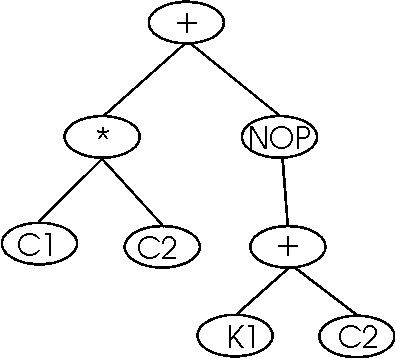
It is possible to create some kind of transformation that will map an existent topology (cyclic graph) into an acyclic graph, without loosing any information, and the converse. Usually, this mapping is one to many (one cyclic graph can be expressed by many acyclic ones, all of the equivalent).
Genetic Programming
The Genetic Programming idea is based in the biological theory of evolution and selection of the fittest. In this theory, the fittest individuals (the ones that performed better) in the present generation, will have a higher probability to reproduce for the next generation. Each generation is composed then with the individuals selected probabilistically (with probability proportional to the fitness) from the previous generation and with mutations or crossovers between these individuals. Usually, the population between generations is kept constant.

In our case, the individuals in a GP run will be the "acyclic graph trees" that are capable of representing a determined "block arrangement" or topology of the construction blocks and their connections.
The GP then will focus on to evolve a "good description" of the solution, but not the solution itself. The outcome will be an acyclic graph that has to be translated into the cyclic graph and then evaluated, but at the time to use the solution, the cyclic graph is the one that is used. We can say that with this approach, the GP evolves a program to write a program that solves our problem. (remember that the mapping is one to many).
In each generation, each evolved program (acyclic tree) has to be translated or compiled into the cyclic graph and then tested to see if it solves the problem (or give a measure of "how close" it is to solve it). The result of this comparison is called the "fitness score" (following the biology language) and is related to the measure of "how much does the output(s) of the evolved program resembles the desired output(s)". This gives us a way to quantify (indirectly) how good are each one of the evolved programs and take decisions based on this. The "template" or "ideal fitness" that is used to compute the final fitness can be composed of several cases (different input/output templates) and the average performance is the fitness score for the individual. This enforces that the fittest individuals accomplish the desired behavior. Also, it gives a good termination criteria, to know when an acceptable individual is found (with an acceptable fitness value).
The programs (individuals) have to be changed between runs. After the fitness score is computed for all the individuals, the fittest are selected to be the base of the next generation. Usually, the population between generations is kept the same. Some of the selected programs are just copied intact. The rest of individuals are derived from the selected individuals performing some operations on them. These operations are usually: mutation and crossover. Mutation takes one individual and changes (in the acyclic tree description) some of the instructions at random (deletes, or introduce new ones), and this is reflected in the topology of the new individual. Crossover takes two (or more) "parent" individuals and copy part of the description of one in the other.
When a new population is created, is then evaluated again and the process keeps going this way until the desired result is found (or the GP decides is time to stop). This can be seen in the Figure 4.
Taking all of this in account then, to solve a problem we have to keep in mind:
- Construction Blocks: What kinds of construction blocks are needed to be used in a topology and find a suitable solution of the problem. The number of construction blocks, and the kind of operations that they perform, the kind and number of input/output and in general all the details involved with the blocks are very important.
- Acyclic Tree Description: Find (decide) an acyclic tree description that can represent ANY allowed block configuration. This is the actual "program" that will be grown by the GP.
- Fitness Function: The grown "acyclic tree descriptions" have to be translated into executable programs (i.e. compiled). Then, each one of these programs is run using one (or several) test input/output sets. With each input set, the real output is compared with the expected one and a score is given. Usually, penalty points are used when the grown system doesn’t behave in the desired way. With this criteria, a score of "0" is a perfect match. With several input/output sets, the average of all the trials is the "fitness score" for that individual. Note that is in this part that the knowledge about the "desired behavior" is introduced. This can be seen as the "training set" in classical non-linear search.
- Selection for the breeding: Selection of the individuals that are going to be copied, mutated or crossed over for the next generation, using a probabilistic approach. The probability of each individual to be selected for breeding should be proportional to their fitness (the better fitness, the more likely to be selected)
- Genetic Operations: Define the mechanism to perform each one of the genetic operations (copy, mutation or crossover) in the acyclic tree descriptions.
- Stop Criteria: Decide when is a good moment to stop and pick a winner.
The first generation of a genetic program is usually composed by "random" programs, and then, the scores obtained in the fitness measurement are very high (a lot of penalty points), and then tend to go down with each generation.
Role of previous knowledge and constrains
Most of the problems have some kind of constrains, especially in the number and kind of inputs and outputs that the grown system or program is expected to have. These are usually incorporated as "default" blocks in each program, and they can’t be modified by the GP. This is one way to force the grown programs to fit a desired interface model.
Implementation of our "toy" problem
Now, let’s talk again about the "toy problem" using the GP language described above and discuss about the implication of all the parts.
The idea is to evolve a "creature" that will wonder around a fictitious world (a grid) with some "food" and "poison". The creature is expected to avoid get stuck with a wall (the boundaries of the squared world), and it will survive if eats as much "food" as possible and no "poison" at all.
The creature can be seen as a "program" that will be run in a simulated environment. The fitness function can be composed of many "random" worlds (in size, and food/poison distribution). Then, each evolved creature is released (the program is run) and tested if the creature ate the food and no poison at all. The programs (creatures) with better performance will survive.
Construction Blocks
The selected platform for this problem was a digital computer, running software to simulate the world, and the creatures on it. The specific computer platform (win, mac, unix, etc) is open. This can be done because we want to evolve higher level commands. The actual implementation will be platform dependent.
With this idea, the construction blocks will be separated in three big categories:
Inputs (sensors): these blocks have no "input" connection. They receive information from the exterior and put a signal in their "output" connection. The proposed input sensors for these creatures are:
- Food Smell: a sensor that gives a signal related to the amount and distance of food.
- Poison Smell: signal related to the amount and distance of poison.
- Touch: signal related to the type of object in front, ie: wall, food or poison.
- Vision: gives a signal if it "sees" food/poison.
Process: these blocks just take input signals and do some processing with them, to put the result at their output.
- Add: add two signals
- Mult: Multiply.
- Split: duplicate a signal (one input, two outputs).
- If: Selection or comparison. If A>B then C. A, B and C are different input signals
Outputs (Actuators): these blocks just have inputs, and they have interaction with the "exterior world". They will respond to control signals and will perform some action.
- Move: will make the creature to advance or move in a pre-determined direction (defined by other control input).
- Eat: Eat the food/poison that is in front.
Acyclic Graph Tree Representation
Because these are the "individuals" that will be evolved by the GP, the selection of a good mapping between the cyclic graph (composed by functional blocks) and the acyclic graph tree is crucial. A bad representation will be one that can not represent ANY block combination. Also, this representation has to be flexible enough, to allow the GP to perform the genetic operations and transformations to it, and the outcome has to be a valid graph that can be then "compiled" and tested for performance.
The components of this graph have to take care of:
- creating the blocks
- connecting (unambiguously) the blocks
- connecting the inputs and outputs (all of them)
These components can be thought as "instructions" of how to assemble a topology (blocks and connections), therefore, they will be called "topology construction functions". Also, some control functions have to be introduced to help the development. They will be called "topology development functions".
To standardize the representation of the multiple kinds of elements that can be present in the graph, we will introduce some conventions:
Number of inputs/outputs. This depends on the type of element. It has a minimum of one input or one output, and a maximum of tree inputs and two outputs. By convention, there is a single connection at the top of the element, and this connection determines the FLOW of the element.
The flow of the element is defined to be UP if the connection on top of the element is an output. The flow is then DOWN (DN) if the connection is an input.
Some elements don't have FLOW, and they are located on top of all the other elements. These will be the "fixed" elements that define the inputs and outputs of the program.
Number of inputs/outputs and flow
Figure 5 shows the convention followed (regardless of the type of element) to number the inputs and outputs, and to name the element taking in account the direction of the flow (that will be very important at the time of making connections or genetic operations).
1 In: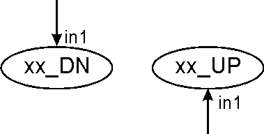
1 Out: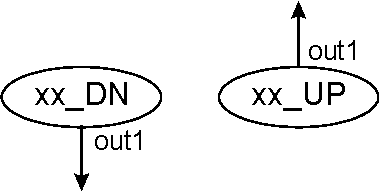
2 In, 1 Out: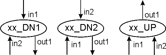
1 In, 2 Out:
3 In, 2 Out: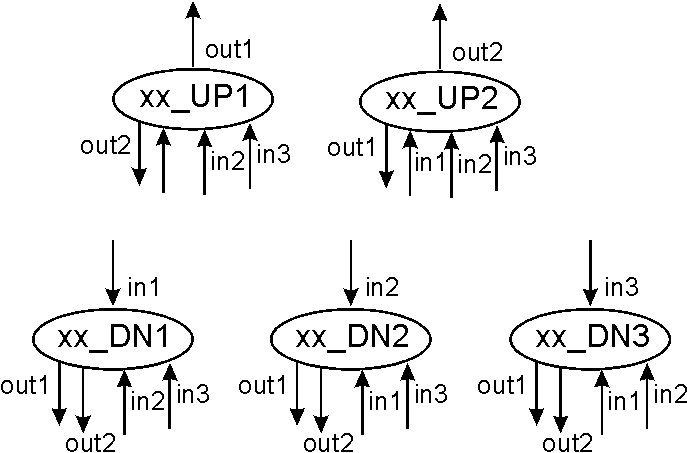
topology construction functions
These functions will introduce a block of the specified type connected to the specified blocks. The representation of each one of these can be found using the guide given in Figure 5, and replacing the xx by the name of the function.
ADD (2 in, 1 out)
Introduces an Addition block. The two inputs are add together and output.
MUL (2 in, 1 out)
Introduces a Multiplication block. The two inputs are multiplied together and output.
SPLIT (1 in, 2 out)
Introduces a Split block. The input is split in two identical copies of itself, and output.
GE(3 in, 2 out)
Introduces a Great or Equal Than block. The operation if(input1>=input2) is performed. If the result is true (input1>=input2), the output1 will output a copy of input3. If the result is false, (input1 < input2), the output2 will output a copy of input3. In both cases, the other output will output a "zero" signal.
KTE(0 in, 1 out)
Introduces a constant in the graph. The output of this element is a constant (that has to be defined by the compiler at runtime). This constant can't be changed during the run of a program.
INPUT(0 in, 1 out)
Introduces an interface with an input sensor. This block reads the actual input of the desired sensor (one sensor per input element) and outputs its value.
OUTPUT(0 in, 1 out)
Introduces an interface with an output actuator. This blocks sends its input to the external actuator (one actuator per output element).
Topology Development Functions
These functions are necessary to control the development of the topology. Some times is important to "freeze" for one moment the execution of some topology construction functions. Also, to be able of representing the loops in the cyclical graph, the introduction of two connection functions is necessary.
NOP (1 in, 1 out)
This function makes the construction of the topology to do nothing in the branch that has it for one time step.
BRIDGE_RX(0 in, 1 out)
This will make a connection with is counterpart (BRIDGE_TX). This functions are very important to connect points very distant in the acyclic graphs.
BRIDGE_TX(1 in, 0 out)
This is the counterpart of BRIDGE_RX.
Connections:
The connections in the acyclic graph tree are translated into connections between blocks in the cyclic graph. These connections have some restrictions, i.e. they flow from one block output to one block input. There can be just one connection per input or output (not multiples connections). The proposed scheme also includes the range of allowed values to be transmitted through the connections to be [-1:1]. In some cases, an operation like ADD will overflow the connection. In this case, an "intelligent" clipping ADD is recommended (that means that if the result is more than one, it is clipped to one, and if is less than -1 it is clipped to -1).
Mapping example:
Example of the mapping from acyclic graph into cyclic graph.
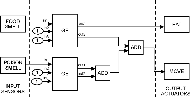
Figure 6 Cyclic graph Example
Figure 6 shows one simple cyclic graph with two input sensors and two output sensors. We set up the input sensors to output a signal of "1" when they sense food or poison, and a signal less than one when they not; and we set up the actuators to move or eat when they receive an input of "1. This graph will work very badly, because the output of the "great or equal than" related with the poison smell, will always output a "1", and make the creature to move, but the creature will just "eat" if it senses food, not poison.
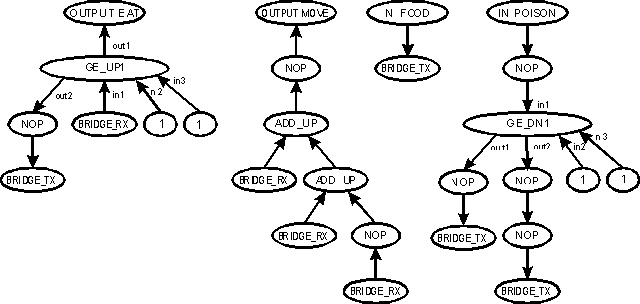
Figure 7 Example Acyclic graph
Figure 7 shows one acyclic graph that can be used to describe the cyclic graph in Figure 6. To use this acyclic graph to re-create the cyclic one, it is necessary to follow some steps (and conventions).
The graph should be read from top to bottom, left to right. An "ellipse" at the top of the graph will represent each output and input. From each one of those ellipses, the graph will start developing, using the topology construction and development functions.
Each level should be interpreted in order from top to bottom, and from left to right. Pay a lot of attention to each pair of "bridge_tx" and "bridge_rx" functions. Remember that their goal is to "connect" two distant points in the cyclic graph. Every time that we find one of those, that point will be connected with the next point that shows the counterpart. This also shows the necessity of using the "nop" (no-operation) function, to prevent some bridge functions to be made in the wrong order.
The whole paper in a nutshell:
Taking the risk of repeat the same information too much, we will summarize the concepts explained and their place into the genetic program process:
The goal is to analyze an approach that can be used to find in an automatic way, techniques that can be used to solve problems. Of course, this approach is narrowed to solve problems in a very known domain (computer program simulations), but it can be expanded to other domains. To help us with this goal, a toy problem (creature eating) is introduced.
Then, some aspects of the "solving" of a problem are discussed, and a special focus in the architecture of the solution is made. The architecture of the solution is the way that the basic elements that we have to solve the problem are going to be combined to achieve the solution. Our goal is to show that the idea of an "open architecture" is a very good approach, even thought that now the problem becomes "to find a suitable architecture that solves the problem".
The idea of the Genetic Programming, with individuals, population, generation, etc is then introduced. But a special emphasis in the necessity of a good "construction block" set, and specially, a good way to describe the topologies of the solution is stated. Also, the problem usually found with the open architecture systems is that they are very difficult to evaluate (compile and run), because they often include loops, recursions and all sorts of parallel process that make their evaluation (and even their development) very difficult.
To help solve this problem, the focus is changed now into the representation of a system in "block form" (cyclic graph), were all the blocks and connections are shown, and the relation between blocks is easy to understand. But they possess the inconvenient that are too difficult to "mutate" or change using the operations necessary to work within a Genetic Program. Then, a mapping between this cyclic graph an a proposed acyclic graph tree is introduced. Note that the final goal is to have a representation of the topologies (that can represent ANY topology) in a way that is suitable for the Genetic Program operations and transformations.
To finish, an example of this mapping is introduced.
References:
[ 1 ] Koza, J. R., Bennett, F.H., Andre, D., Keane, M.A. Genetic Programming III Darwinian Invention and Problem Solving, Morgan Kaufmann Publishers, San Francisco, CA, 1999
[ 2 ] Koza, J. R., Bennett, F.H., Andre, D., Keane, M.A. Automated Synthesis of Analog Electrical Circuits by Means of Genetic Programming, IEEE Transactions on Evolutionary Computation, Vol. 1. No 2. July 1997.
[ 3 ] Digital Biology Website: http://www.digitalbiology.com/
[ 4 ] The Genetic Programming Notebook, by Jaime A. Fernandez. http://www.geneticprogramming.com/
[ 5 ] UCLA Artificial Intelligence. http://www.cs.ucla.edu/csd/fields/ai.html